Overview

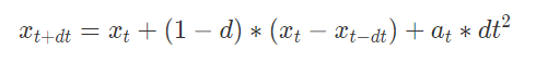
In project 4, we simulate the motion of cloth in realistic settings. In part 1, we create our cloth as a grid of masses with springs (of types structural, shearing, and bending) between them for our model. In part 2, we calculate the forces experienced by each point mass. First, we calculate the external force experienced by the point masses, and then add each point mass’ individual spring correction forces to those external forces; this gives us the force experienced by each point mass at any given timestep. Next, we use Verlet integration to compute new mass positions at each time stamp using the equation:

and constrain the positions by not allowing the springs to extend to more than 1.1 times their rest length. In part 3, we handle the way our cloth interacts/collides with spheres and planes by not allowing them to clip through them and instead applying a repellant force upon collision, and we also account for friction. In part 4, we handle self-collision of our cloth in a sped up fashion by hashing our cloth’s points and comparing each point’s location to other points within the same hash region. In part 5, we implement accelerated shaders by implementing diffuse shading, Blinn-Phong shading, texture mapping, displacement/bump mapping, and finally environment-mapped reflections.

Part 1: Masses and springs

In this part, we separate our code into two parts: when orientation is HORIZONTAL, and when orientation is VERTICAL. In both, we have a nested for loop iterating first over height and then over width. When it’s HORIZONTAL, our iteration is over the x-z plane, and we set our y to be a fixed 1. For each point, we test for if it’s pinned, and then place that point into point_masses. If it’s VERTICAL, we’re instead iterating over the x-y plane, and we set our z value for each point to a random value between -1/1000 to 1/1000 by creating a random value from -1000 to 1000 and then dividing it by 1000000. We then perform the same operations as in the HORIZONTAL case. Then, for the springs, we divide into the three classes: structural, shearing, and bending. For each one, we have two nested for loops to iterate through the entire cloth. For structural, the first nested for loop is for the point on the left of each point, and the second is for the point above each point. For shearing, the first is for the point to the top left, and the second is for the top right. For bending, the first is for the point two to the left, and the second is for two above. Our problem initially was in how we were calculating our random number, as it generated problems for our part 4 cloth rendering. We were able to overcome this by changing how we were calculating my_rand, performing it divided by 1000000 as opposed to 1 over it.

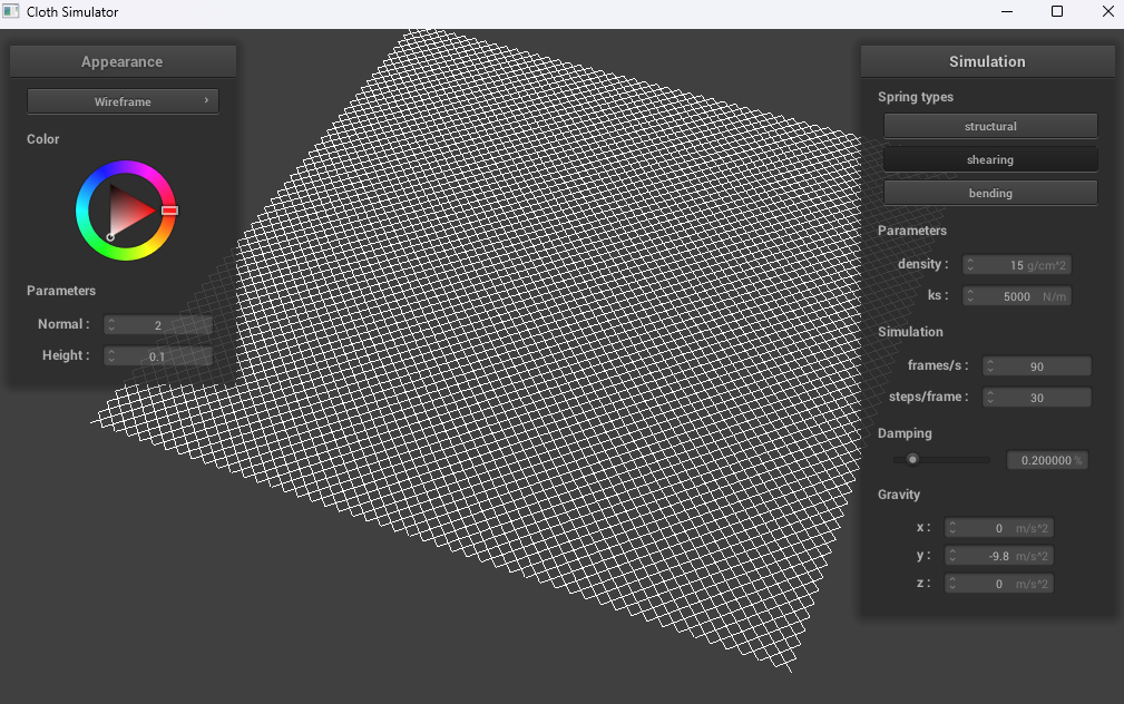
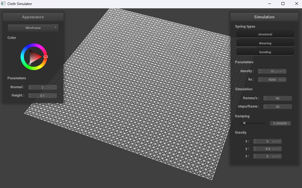
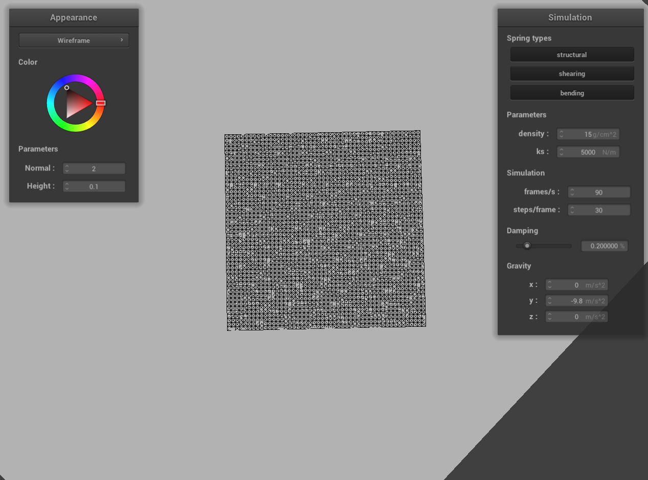
Take some screenshots of scene/pinned2.json from a viewing angle where you can clearly see the cloth wireframe to show the structure of your point masses and springs.

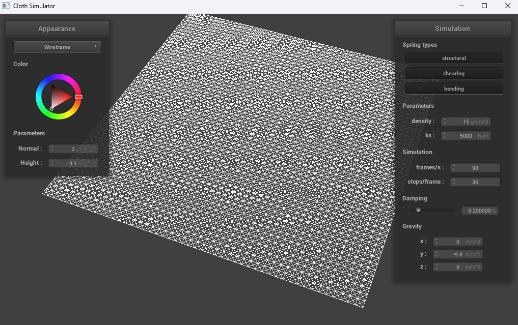
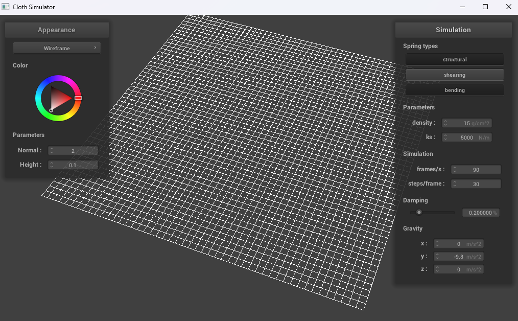
Show us what the wireframe looks like (1) without any shearing constraints, (2) with only shearing constraints, and (3) with all constraints.

Part 2: Simulation via numerical integration

We began with calculating the total external force of each point mass. Then, we took in consideration the spring correction forces. We took that into account in order to calculate the total force that is exerted on each of the point masses. We made sure that the bending constraint was weaker than the shearing and the structural constraints. Then, we used Verlet integration to compute the new point mass’s position in order to keep the points up to date. One part that we had to make sure to be careful of is that we needed to make sure that we used the total force exerted on the point mass instead of just the external forces when calculating the new position of the point mass. Lastly, we made sure that after each position update, the two point masses’ positions were at most 10% of the rest length. If one of the point masses is pinned, then we do not move that point mass, and if they are both not pinned, then we move both point masses with the same amount.

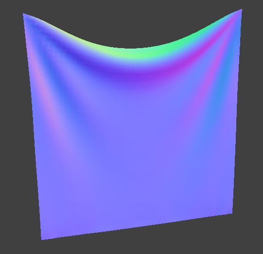
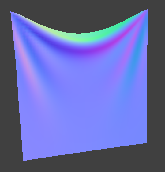
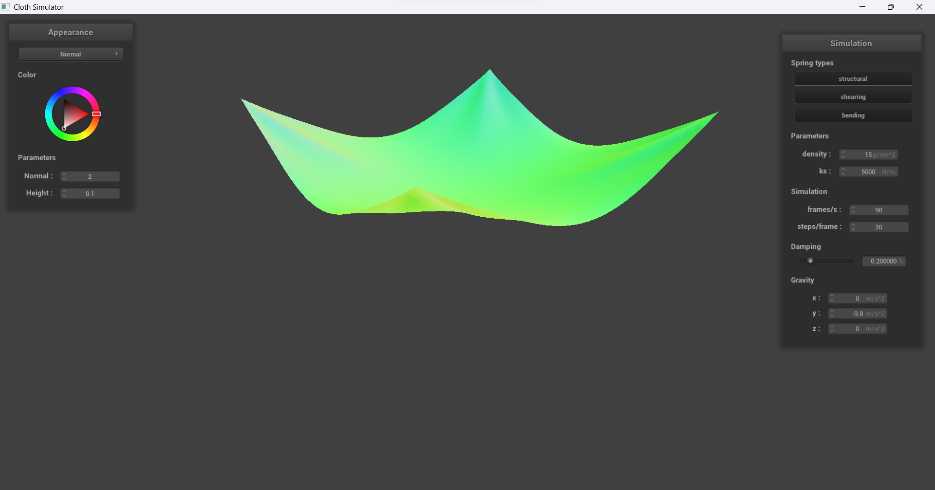
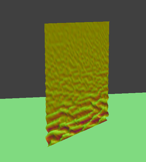
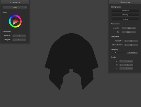
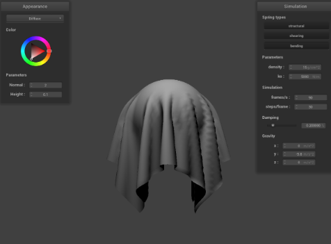
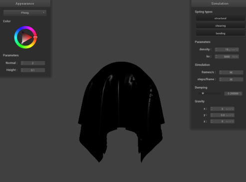
Experiment with some the parameters in the simulation. To do so, pause the simulation at the start with P, modify the values of interest, and then resume by pressing P again. You can also restart the simulation at any time from the cloth's starting position by pressing R. Describe the effects of changing the spring constant ks; how does the cloth behave from start to rest with a very low ks? A high ks? What about for density? What about for damping? For each of the above, observe any noticeable differences in the cloth compared to the default parameters and show us some screenshots of those interesting differences and describe when they occur.

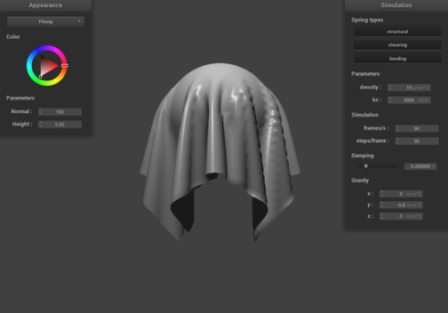
If we change the values of the spring constant ks, we’re changing how different “parts” of the cloth interact with each other. With a very low ks (we took 1 N/m), the spring force between any two given “points” on the cloth is much smaller than the external force(s) on the cloth, meaning that the spring force is almost invisible to the naked eye; this results in a cloth that falls completely flat with no visible creases. In the middle, at the default ks (5000 N/m), we see more of the springs’ effects on the cloth with more self-interactions in the cloth that result in more creases. On the other hand, when we have a very high ks (we took 99999 N/m), the spring forces become much more prevalent and create a “bouncing” effect as the cloth’s “points” continuously experience strong pushing and pulling forces. This results in a much more upright final position, with the cloth sagging less and less as our spring constant increases.

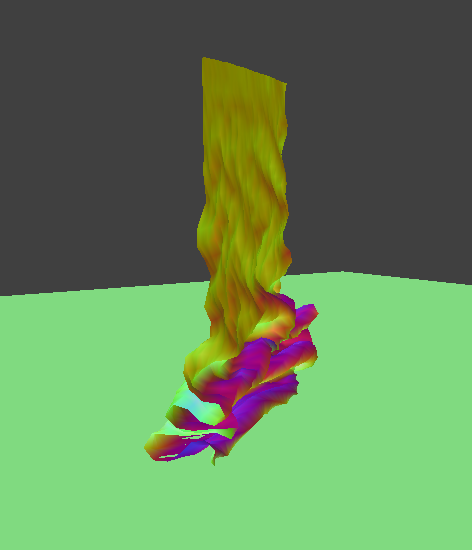
When changing the density, with extremely low densities (like 1 g/cm^2), we have a rather light cloth with light “components,” so we don’t see as many creases. At an intermediate point of density (such as the default 15 g/cm^2), we have more creases since the points experience more forces with their increased density and thus mass. With an extremely high density (99999 g/cm^2), the force of gravity on the “points” of the cloth becomes too great, and so the now-heavy cloth falls flat. Overall, the greater the density, the more the cloth will sag down.

Finally, with damping, we can change how we simulate conservation of energy in our system. With a damping of 0%, our cloth seems to exhibit a model of conservation of energy with no energy lost to heat/friction/sound/etc., so it continues to swing back and forth seemingly endlessly. At a damping of the default 0.20%, we see a more realistic simulation of the cloth falling, as it loses some of its energy to heat/friction/sound/etc., meaning that the potential energy isn’t always fully converted to kinetic energy. This results in the cloth falling to an eventual rest, but not before experiencing some form of a “swinging” back and forth. At a damping of 1%, the cloth falls more slowly since its kinetic energy becomes quickly lost, resulting in it not being able to build up a fast speed. Our cloth here will fall to a resting state on its first “swing” immediately.

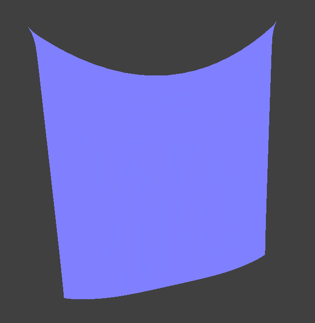
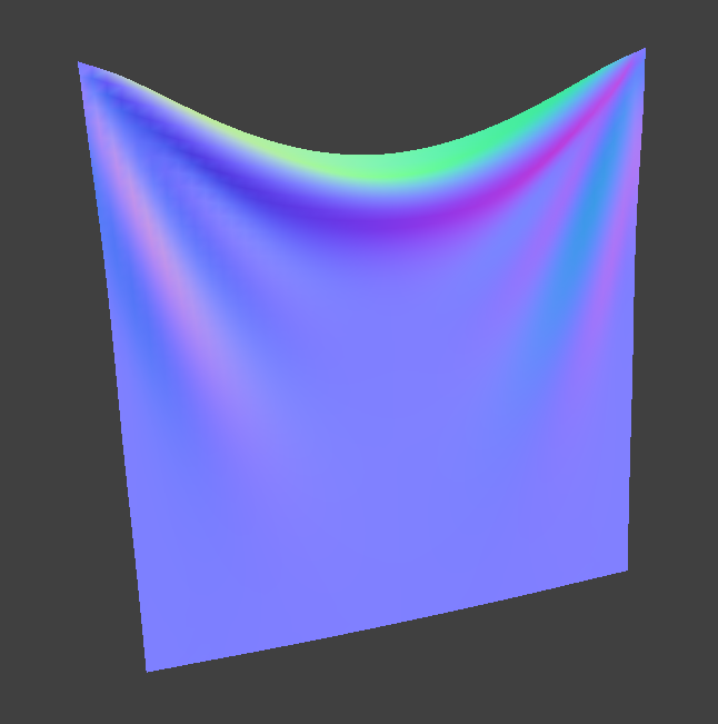
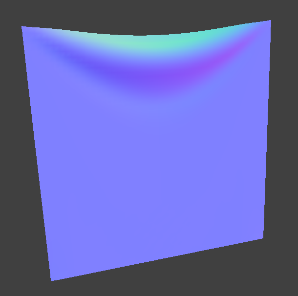
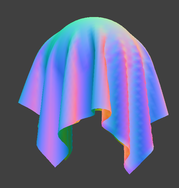
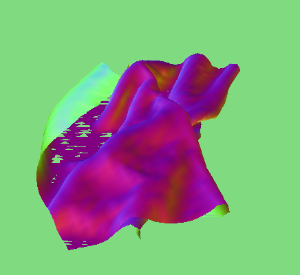
Show us a screenshot of your shaded cloth from scene/pinned4.json in its final resting state! If you choose to use different parameters than the default ones, please list them.

Part 3: Handling collisions with other objects

For collision with spheres, we first got the distance between the position of the point mass and the origin of the sphere. If the point mass’s position is within the radius of the sphere, then we change the point mass’s position to a little bit outside the sphere by getting the total distance towards the same direction of the point mass’s position and moving it by a little bit by scaling it with friction force. For this part, we had no trouble getting through it. For collision with a plane, we did the same thing as a sphere, but we used the ray-intersection with plane equation to make sure that the point mass's position was above the plane and it says above the plane. If the point mass’s position gets closer to the plane, then we make sure to change the point mass’s position such that it will stay above the surface of the plane. For this, our cloth was falling very slowly, so we made sure that the t value that is the constant that is getting multiplied by the vector is low enough for the point mass’s position to change. Other than the cloth falling down too slowly, we did not have a problem with this part.

Show us screenshots of your shaded cloth from scene/sphere.json in its final resting state on the sphere using the default ks = 5000 as well as with ks = 500 and ks = 50000. Describe the differences in the results.

I believe the difference is that ks determines how stiff the cloth is. If the ks value is higher, the cloth becomes stiffer which means that the cloth will not follow the shape of the object. If the ks value becomes lower, the cloth becomes more flexible and follows more of the structure of the object compared to a higher ks value.

Show us a screenshot of your shaded cloth lying peacefully at rest on the plane. If you haven't by now, feel free to express your colorful creativity with the cloth! (You will need to complete the shaders portion first to show custom colors.)

Part 4: Handling self-collisions

For this part, we had a problem with the build_spatial_map because we did not know how to build the spatial map because it had like vector*, but I did not know how to add point mass to this vector, so it took us a while to figure this out. We asked classmates about this part, and we were able to figure it out. Then, self-collide was a bit of a problem because we thought that we had the code correct for this part, but when we changed the variables such that it was easier to read, it worked. We think that this was a problem on our part because we kept reusing the variables instead of just creating a new variable for our calculation. Our hashing was good from the start, so we were fine with the hashes.

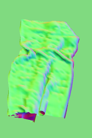
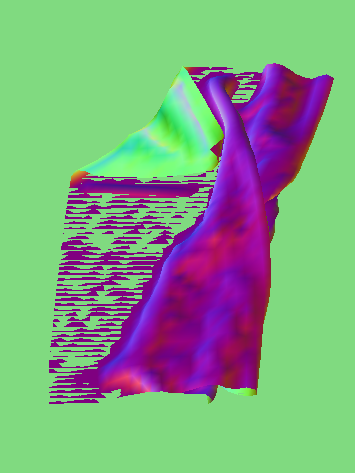
Show us at least 3 screenshots that document how your cloth falls and folds on itself, starting with an early, initial self-collision and ending with the cloth at a more restful state (even if it is still slightly bouncy on the ground).

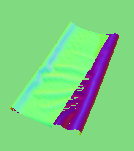
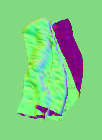
Vary the density as well as ks and describe with words and screenshots how they affect the behavior of the cloth as it falls on itself.

Starting with the ks values, higher ks value makes the cloth more rigid so that when it falls down, it does not like to be together in one place compared to a lower ks value. When the ks value is high, the cloth tries to spread out more quickly, and when it comes to a rest position, it has less folds and less arches. Lower ks value tends to act the exact opposite of a high ks value. Next, for the density, higher density seemed like the cloth felt more heavier such that the cloth actually did not shift around that much from the time when the cloth fell to the plane up until its rest state. Lower density seemed like the cloth was more bouncy and it moved around way more compared to the higher density cloth. It also took longer for it to be stable as well.

Part 5: Cloth Sim

For diffuse shading, we used the equation given to us by the specs, but we set the kd as (1.0, 1.0, 1.0) because that was what it was recommended in Ed. Then, we calculated the “r” variable by getting the distance from the light source’s position to the output vector’s position. Then, for n, we had to normalize the normal vector in order for the diffuse lighting to work. For Blinn-Phong Shading, we set the ka, kd, ks, Ia, and p to the recommended numerical values from Ed. Then, the rest of the calculation just followed the steps for Diffuse shading. We were a bit confused about this part because the kd values were a vector for the diffuse shading, but for Phong shading, it was a float value. We were able to resolve this conflict by looking through ed and understanding why it works with both vector and float values. Texture mapping and Environment-mapped Reflection was straightforward as we just used the texture built-in function. For bump mapping, we calculate our dU and dV with our texture coordinates and our width and height, then use an application of the TBN matrix for our new normal vector to use. For displacement mapping, we take what we had from bump mapping and change the position by n*h(u,v)*k_h.

Explain in your own words what is a shader program and how vertex and fragment shaders work together to create lighting and material effects.

A shader program allows for renderings of realistic lighting to run in parallel to speed up the runtime of our program. Vertex shaders change properties of the vertices (position, normal vectors, etc.), and fragment shaders take in the fragments’ attributes from the vertex shader to compute the color.

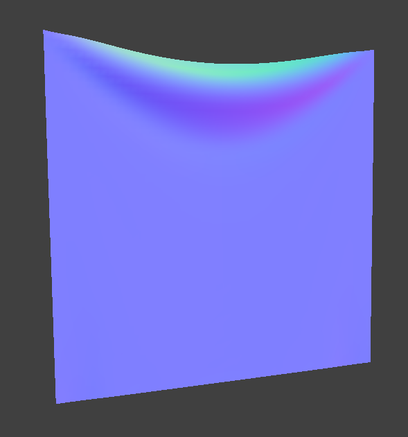
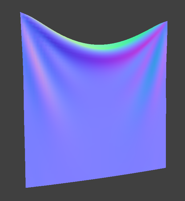
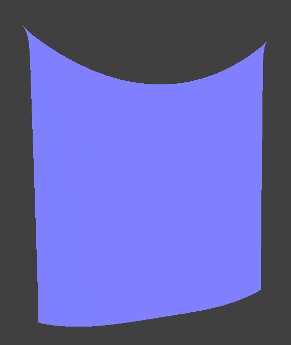
Explain the Blinn-Phong shading model in your own words. Show a screenshot of your Blinn-Phong shader outputting only the ambient component, a screen shot only outputting the diffuse component, a screen shot only outputting the specular component, and one using the entire Blinn-Phong model.

For Blinn-Phong shading, we took into consideration of the ambient light component and specular reflection component to the diffuse lighting to create a more realistic view of the sphere over the cloth because only with the diffuse lighting, it does not recreate the realistic view, and with the ambient light and specular reflection component, it shows more realistic view. With Blinn-Phong shading, as we took into account the angle between the source position and the surface normal, as well as the light source position, we were able to create a more realistic and accurate real life image.

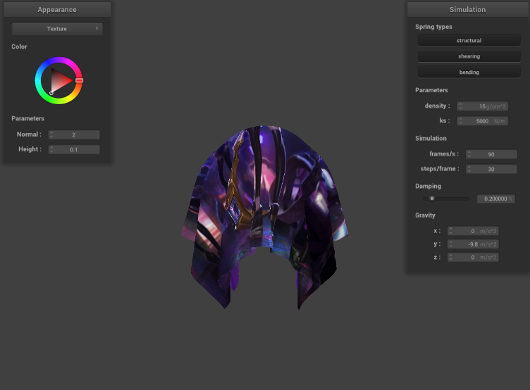
Show a screenshot of your texture mapping shader using your own custom texture by modifying the textures in /textures/.

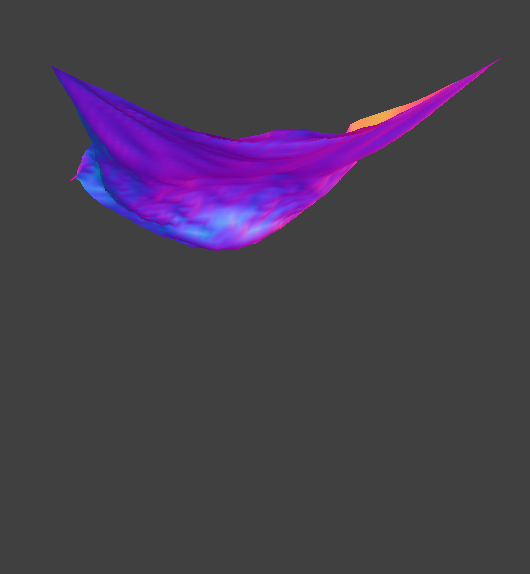
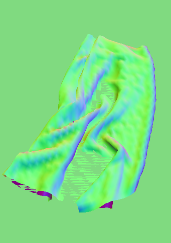
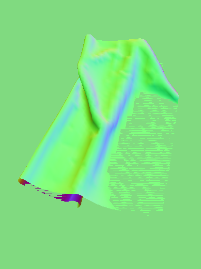
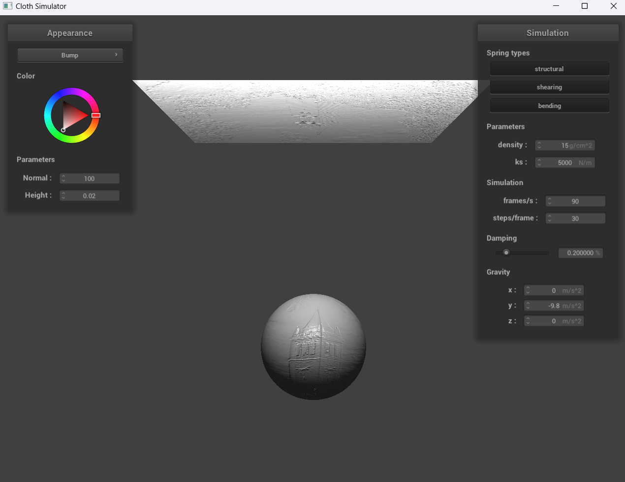
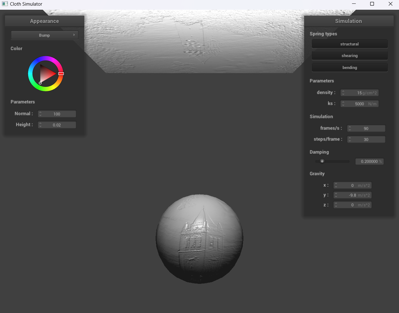
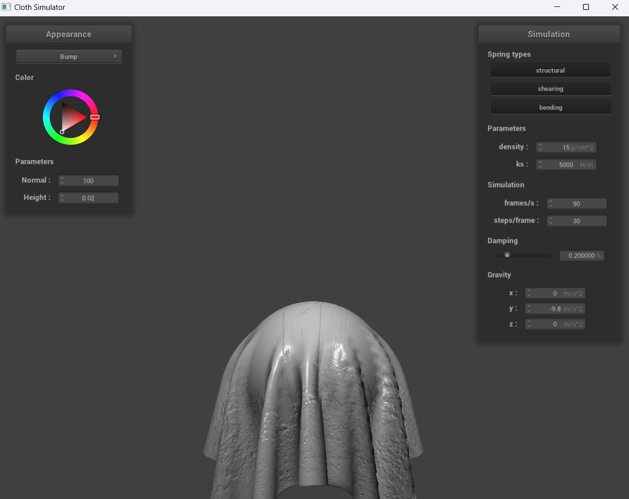
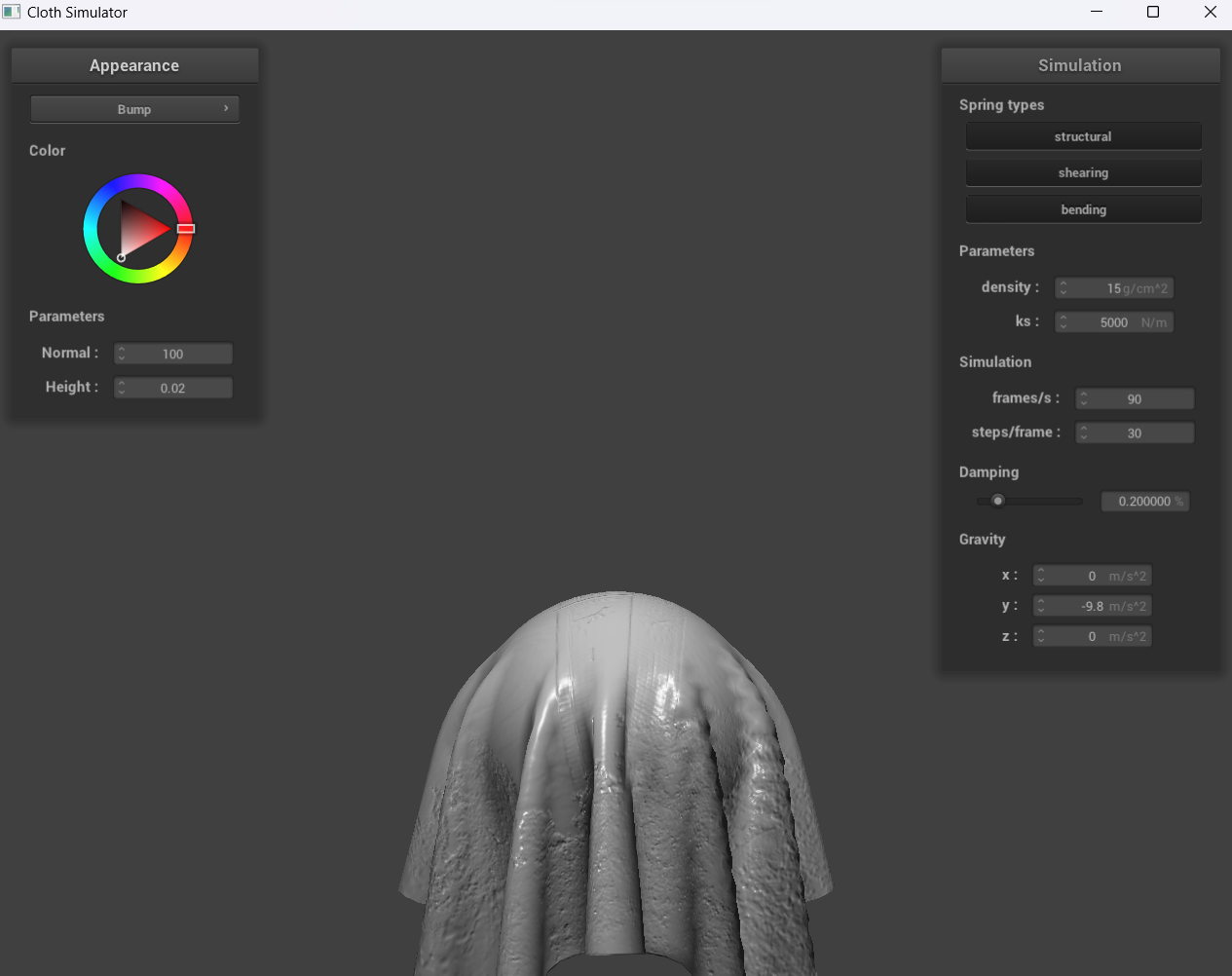
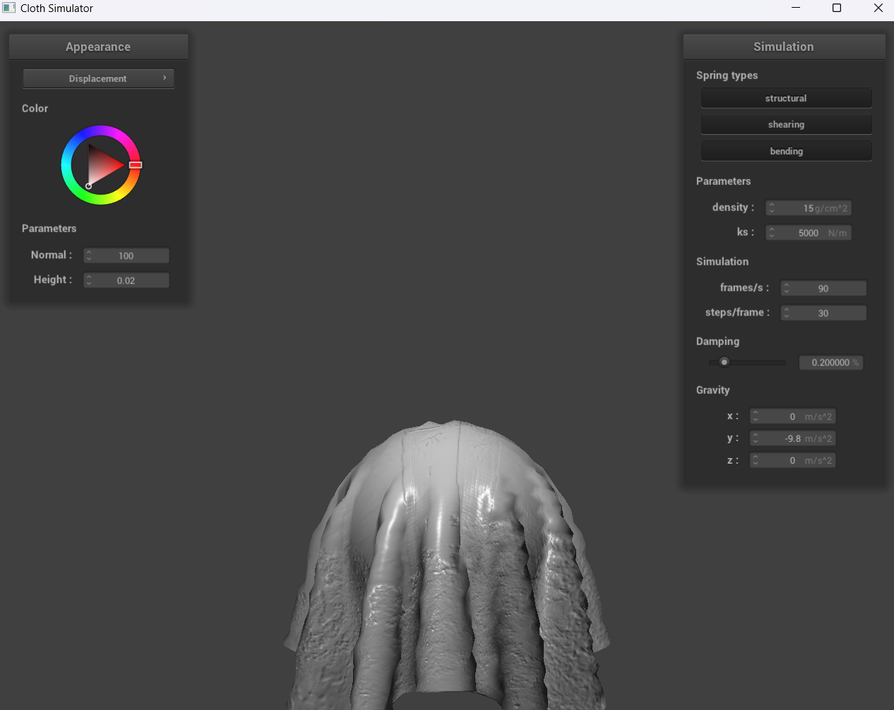
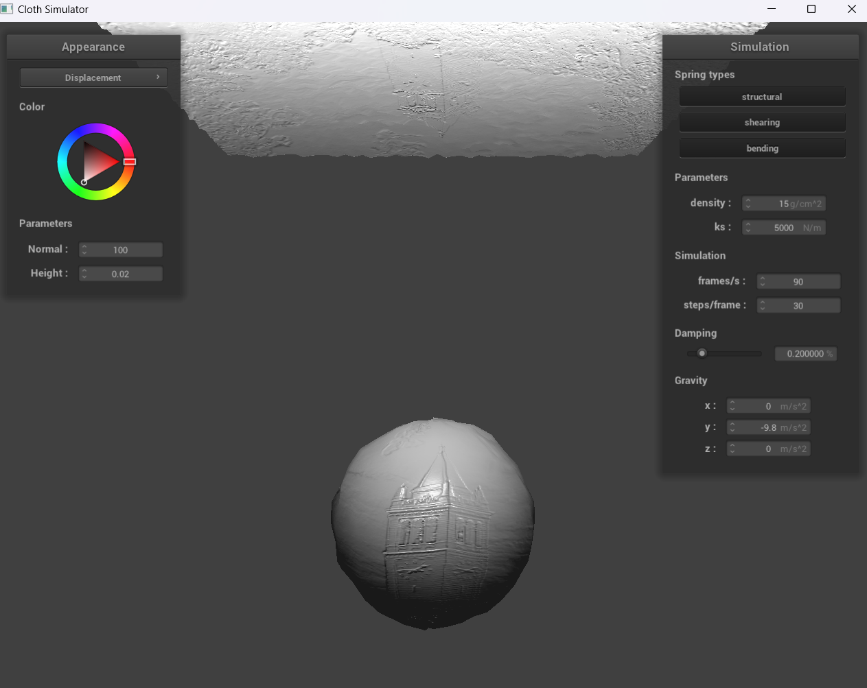
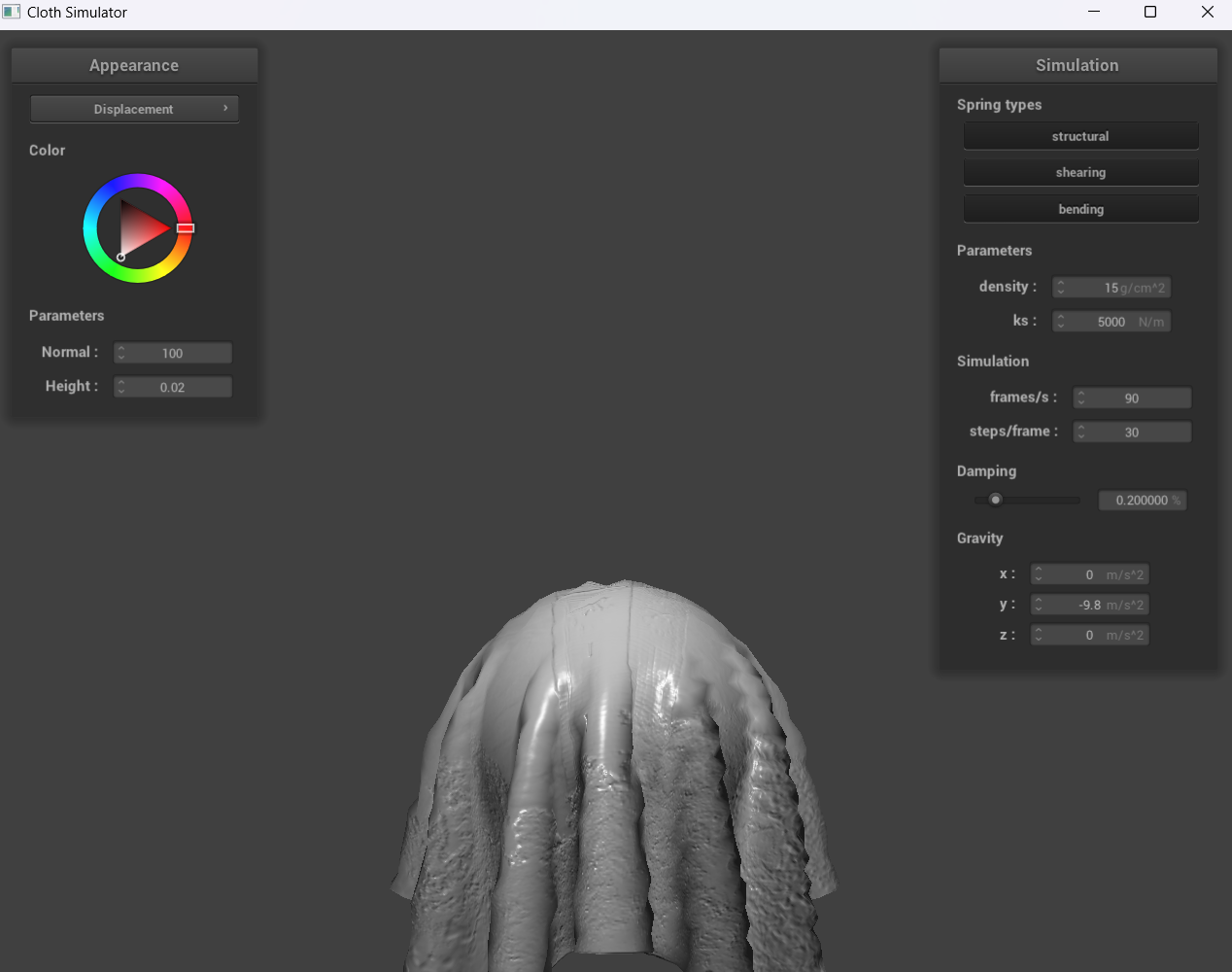
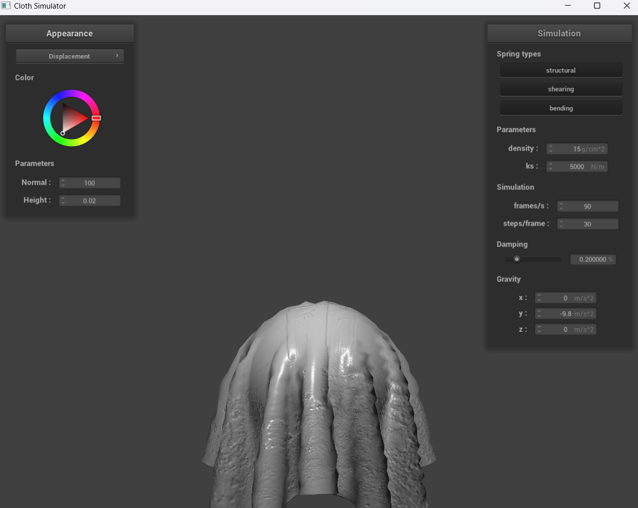
Show a screenshot of bump mapping on the cloth and on the sphere. Show a screenshot of displacement mapping on the sphere. Use the same texture for both renders. You can either provide your own texture or use one of the ones in the textures directory, BUT choose one that's not the default texture_2.png. Compare the two approaches and resulting renders in your own words. Compare how your the two shaders react to the sphere by changing the sphere mesh's coarseness by using -o 16 -a 16 and then -o 128 -a 128.

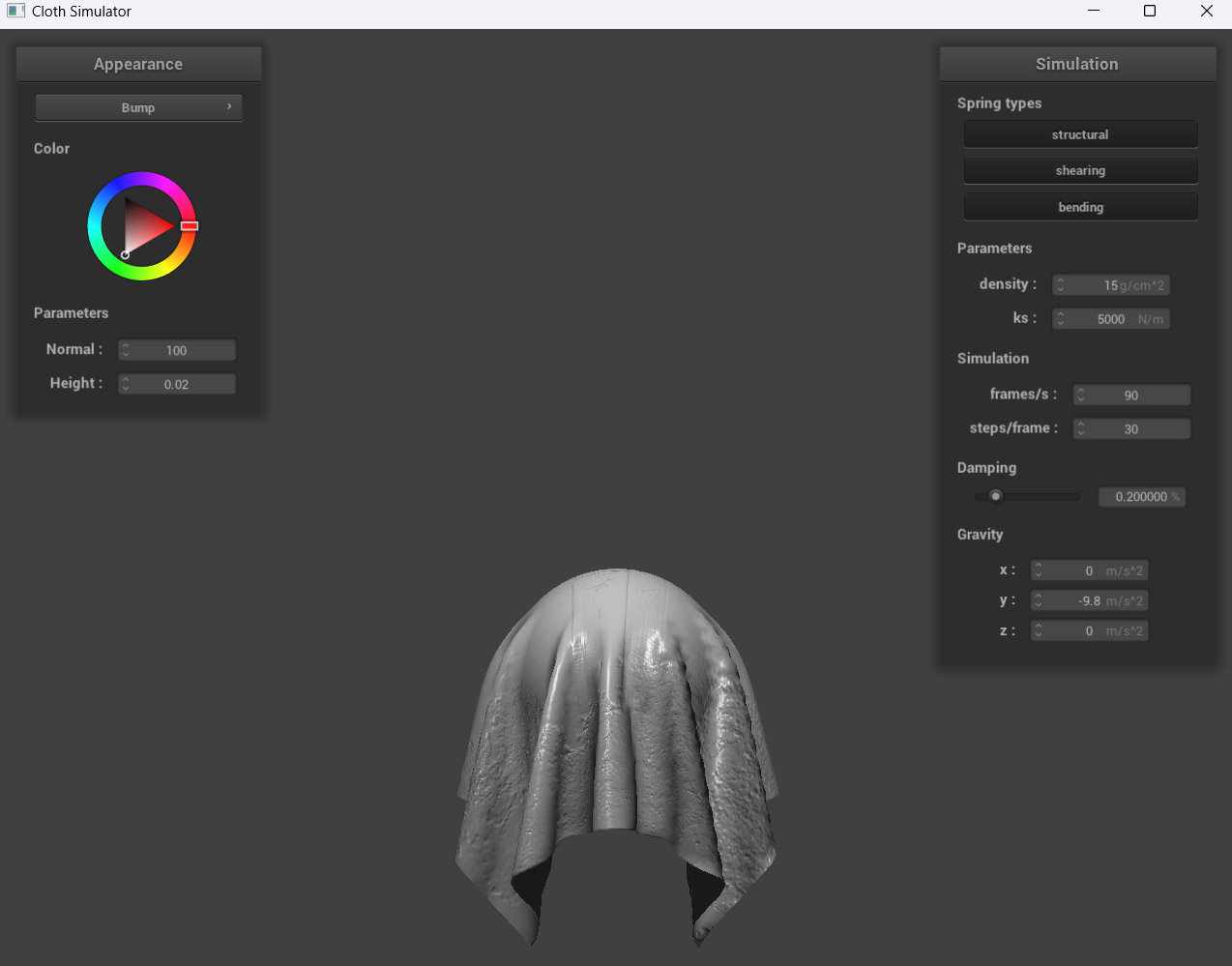
With bump mapping, the normal vectors of our object are modified to make it appear as if details (through the bumps) are present. On the other hand, with displacement mapping, the normals are modified and the vertices have the position changed for the height map.

For displacement mapping, our sphere is evidently much bumpier than the sphere in bump mapping, and once the cloth falls down, the folds for displacement mapping are also larger. Furthermore, when we change the sphere mesh’s coarseness, the image we see with -o 128 -a 128 is clearer than -o 16 -a 16.

Show a screenshot of your mirror shader on the cloth and on the sphere.

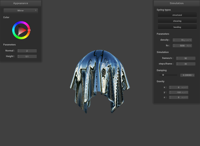
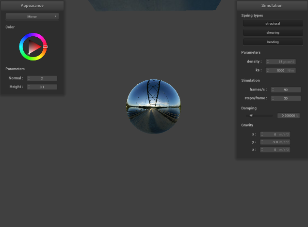
Explain what you did in your custom shader, if you made one.

N/A

Partner

For this project, we worked on the parts together by meshing together our ideas, allowing us to debug our code quickly whenever we came across them. One problem we had was that we weren’t sure if the construction of our grid of point masses with their springs in part 1 was correct, so whenever we ran into a bug, we weren’t sure if the bug was in that part or actually just in part 1. Part 5 also was interesting for us as it felt like it had more of a connection to previous projects. Overall, this project was very beneficial for us as we learned how to build a physics simulation from start to finish, which is what we plan on doing for our final project.