Overview

For each part of this project, we looked at the reference slides to get most of the information needed in order to have the correct logic for our code. We began this project with just a simple generation of ray. With the ray, we checked if a ray intersected with a triangle or a sphere by using Moller Trumbore algorithm, and sphere intersection equation respectively. Secondly, we implemented a bounding volume hierarchy to make the rendering faster and optimize the ray-surface intersection process. By implementing this part, we were able to render an image with hundreds of thousands of triangles in only a couple seconds. Next, we implemented the illumination for zero bounce, one bounce, and at least one bounce radiance. For the one bounce radiance, we used Monte Carlo Integration to calculate the outgoing light. With these functions implemented, each image would take around a whole minute to render which is very long compared to before. Lastly, we implemented a very simple algorithm to enable adaptive sampling. With this implementation, we can see where there are high and low sampling rates which is pretty cool!

In the process of implementing these functions, we have encountered many problems such as getting a single color for rendering a cow after implementing the bounding volume hierarchy, but we were able to solve it by noticing the problem was from normal_shading. Another problem that we had was that we were getting very dark images after implementing the at_least_one_bounce_radiance function. We were able to debug through this rendering problem by talking with peers as well as checking on previous intersection implementation of spheres.

Part 1: Ray Generation and Scene Intersection (20 Points)

Walk through the ray generation and primitive intersection parts of the rendering pipeline.

For generating rays, we first convert the cartesian coordinates onto the canonical sensor plane. We normalize the converted vector, then multiply it by the c2w vector, then normalize it again to find the normalized world_ray vector. To generate the pixel samples, we iterate through num_samples, and get a camera’s ray vector with some random noise. Then, we take the sum of all of the estimates of the rays in the scene, then at the end, divide it by the num_samples to get the average value of it.

Explain the triangle intersection algorithm you implemented in your own words.

Our triangle intersection algorithm first uses has_intersection which we use Moller Trumbore Algorithm to get the following values, {t, b1, b2}. With the values that we get, we check for their bounds such as t being in between r.min_t and r.max_t, and have b1, and b2 in between 0 and 1 inclusive. We return true if all the constraints satisfy, and if not, we return false. In the intersect function, we use has_intersection to check if there exists an intersection between the triangle and the ray. If there happens to be an intersection, we use the Moller Trumbore Algorithm, again, to find {t, b1, b2} values. We check if the t value is less than r.max_t, and if it is, then we perform r.max_t = t. We can use {1- b1 - b2, b1, b2} along with {n1, n2, n3} to find the surface normal at the intersection. If it has an intersection, we return true, and if not, we return false.

Show images with normal shading for a few small .dae files.

Part 2: Bounding Volume Hierarchy (20 Points)

Walk through your BVH construction algorithm. Explain the heuristic you chose for picking the splitting point.

Our BVH construction algorithm has the base case of when the number of primitives in our current node is less than or equal to max_leaf_size, since any node with leaf count of no more than max_leaf_size must be a leaf. In this base case, we simply return our node containing primitives from start to end. Otherwise, we use a heuristic to determine which of the x-, y-, and z-axes we should split our remaining primitives across (splitting in half at the weighted centroid of that axis), and then recursively call the function again on the left half of the primitives and the right half of the primitives. Our heuristic is taking max+min-2*avg, which takes the distance between the maximum and the average and weights it heavily while providing a negative weight to the distance from the minimum to the average. This way, we strongly value one side’s variance and choose the axis that has a stronger skew for our recursive call in that iteration.

Show images with normal shading for a few large .dae files that you can only render with BVH acceleration.

Compare rendering times on a few scenes with moderately complex geometries with and without BVH acceleration. Present your results in a one-paragraph analysis.

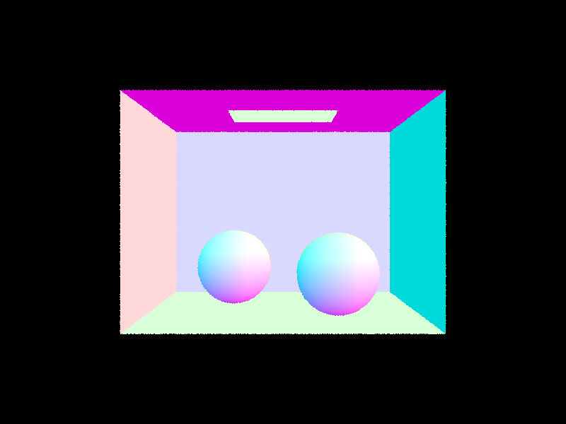
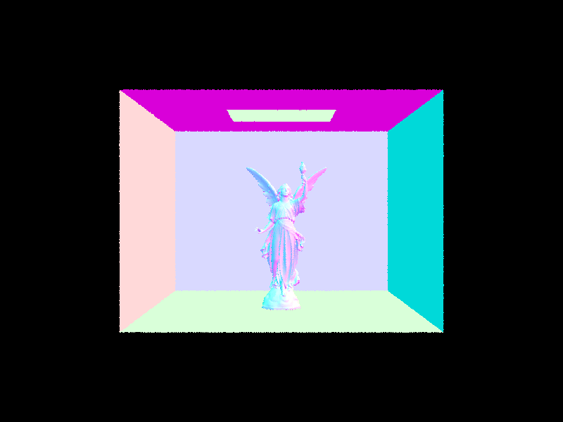
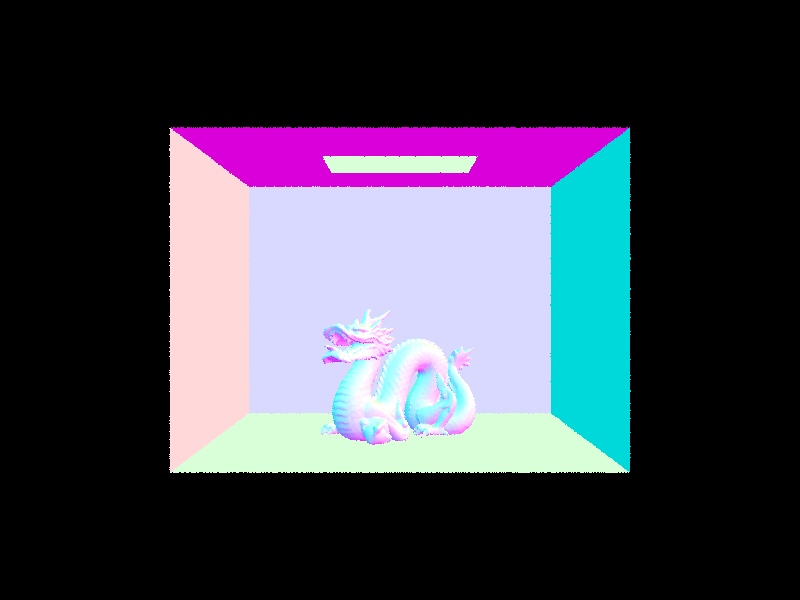
For CBspheres.dae, we see a very small increase in performance from 0.3497s to 0.2768s. However, when we get to cow.dae, we see a larger dropoff from 44.1443s to 0.1219s. With our third comparison of CBcoil.dae, our dropoff goes from a staggering 100.7003s to a mere 0.4254s. We see that in the files with moderately complex geometries, the rendering time with BVH acceleration becomes drastically improved compared to without BVH acceleration. This is because BVH acceleration allows us to eliminate calculations in cases where the ray does not intersect with the surface. By using BVH acceleration, we’re able to generate images with tens of thousands to hundreds of thousands of triangles, such as CBlucy.dae, CBdragon.dae, maxplanck.dae, and peter.dae.

Part 3: Direct Illumination (20 Points)

Walk through both implementations of the direct lighting function.

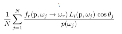
In the estimate_direct_lighting_hemisphere function, we iterate through the num_samples, and for each iteration, we first check if the new ray going from hit_p in the sampled direction intersects with the light source. If it does intersect, we take the bsdf of wi and w_out, emission, pdf as 1/(2*PI) to use the following formula to calculate the outgoing light. Final point, we only do this calculation if cosine is positive.

The estimate_direct_lighting_importance function is very similar to estimate_direct_lighting_hemisphere, but instead of having a set num_samples, we have to iterate through each of the light sources. During each iteration, we also want to iterate through ns_area_light to get the outgoing light. The calculation for outgoing light is the same as estimate_direct_lighting_hemisphere. After getting the outgoing light through ns_area_light iteration, we want to sum them with all the other iterations of the light source. Overall we are still using the Monte Carlo estimator, but we are just going through more for loops. Just a side note, when is_delta_light() returns true, we know that the light is coming from a point light source, so we can just set num_samples = 1 to save some time when we render an image.

Show some images rendered with both implementations of the direct lighting function.

Focus on one particular scene with at least one area light and compare the noise levels in soft shadows when rendering with 1, 4, 16, and 64 light rays (the -l flag) and with 1 sample per pixel (the -s flag) using light sampling, not uniform hemisphere sampling.

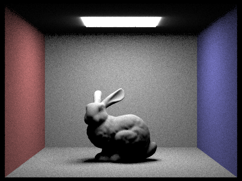
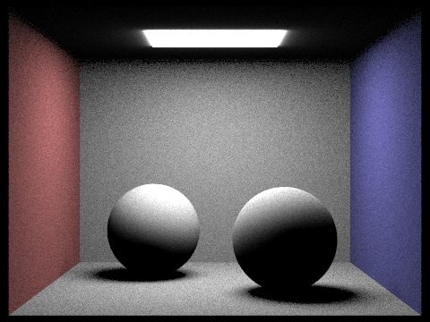
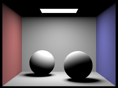
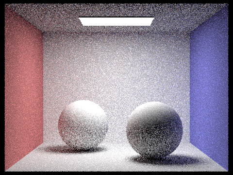
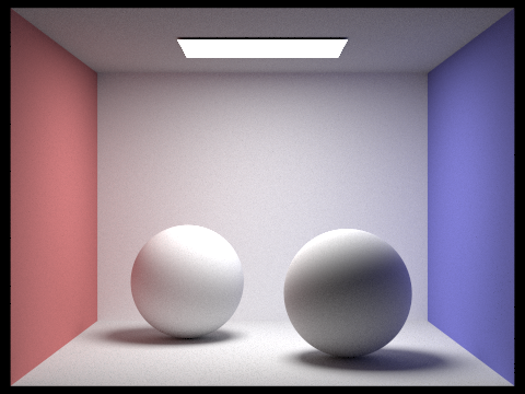
As the number of light rays increases, we can notice that there is less noise in the images. I think this is because with the importance_sampling, the more light there is, the better the quality becomes.

Compare the results between uniform hemisphere sampling and lighting sampling in a one-paragraph analysis.

Comparing the hemisphere sampling with the importance sampling, hemisphere sampling gives us more of a grainer image because we are taking samples from all directions around a single point. However, importance sampling prioritizes samples that contribute more to the result. This is done by sampling and integrating over from only the lights which can make sure that we are only taking samples from angles where incoming radiance is non-zero. This results in a much smoother image.

Part 4: Global Illumination (20 Points)

Walk through your implementation of the indirect lighting function.

For our indirect lighting function, at_least_one_bounce_radiance, we had an initial check of the ray’s depth such that if it was 0, we would return a zero vector. If the ray depth is not 0, then we want to use one_bounce_radiance to have a guaranteed bounce within the function. After the guarantee bounce, we want to calculate the new ray. Before we continue with the russian roulette, with the newly generated ray, we want to make it one less depth than the current ray. Then, perform russian roulette to see if we want to continue the bounce. If we pass the russian roulette probability, we want to check if the new ray still intersects, and if it does, we do a recursive call on at_least_one_bounce_radiance with the inputs as the new ray and new intersection and sum the outgoing lights together. As always, we multiply and normalize the result. If it does not pass the russian roulette, we just return the outgoing light.

Show some images rendered with global (direct and indirect) illumination. Use 1024 samples per pixel.

Pick one scene and compare rendered views first with only direct illumination, then only indirect illumination. Use 1024 samples per pixel. (You will have to edit PathTracer::at_least_one_bounce_radiance(...) in your code to generate these views.)

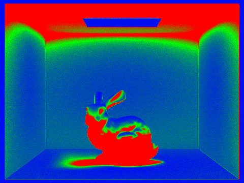
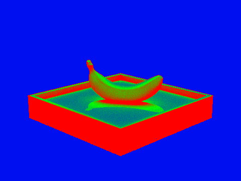
Here, we have direct acting as the light’s direct impact on our room, and indirect acting as the light’s reflections across the room. In general, global lighting is the sum of our direct and indirect lightings.

For CBbunny.dae, compare rendered views with max_ray_depth set to 0, 1, 2, 3, and 100 (the -m flag). Use 1024 samples per pixel.

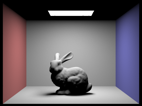
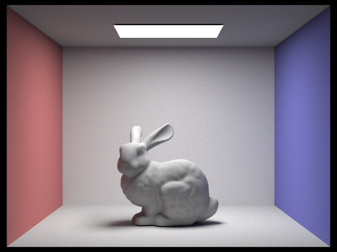
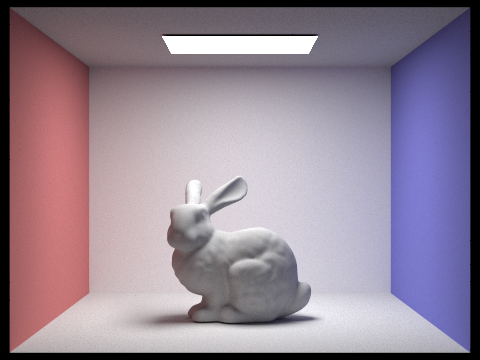
At m=0, we see that there are no reflections, as it is only radiance in effect. Then, at m=1, we see the direct effect of the light on the room. At m=2, we begin to see a brighter room with a greater maximum ray depth, and from there, on paper, it’d be brighter, but the images begin to look similar.

Pick one scene and compare rendered views with various sample-per-pixel rates, including at least 1, 2, 4, 8, 16, 64, and 1024. Use 4 light rays.

As we have higher sample-per-pixel values, we see less dots since as we sample more, we will have less noise in our results. This results in the clearer, crisper images in the higher sample rates.

Part 5: Adaptive Sampling (20 Points)

Explain adaptive sampling. Walk through your implementation of the adaptive sampling.

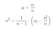
Adaptive sampling allows us to sample less on locations that converge early on to their correct value. We take I =1.96* n for measuring the convergence on a specific location, where the 1.96 comes from our 95% confidence interval, sigma is the standard deviation of our samples thus far, and n is how many samples we’ve taken. Our test for convergence is done by testing if I≤maxTolerance*, where maxTolerance is some predetermined value and mu is the mean of our samples thus far. This can be thought of as I becoming smaller and thus converging when either sigma is small and thus we have a smaller 2 for our variance (meaning all values are similar) or the number of samples is large and we have found an adequate convergence.

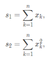
Our implementation is done by adding onto our previous code for raytrace_pixel(). We introduce variables of s1, s2, sig, mu, I, and my_samples for the calculations. While iterating through our number of samples ns_aa, we calculate the illumination of our ray and add them to s1 and s2 to use the following equations:

Then, after every samplesPerBatch samples (which we test for by taking the mod of my_samples against samplesPerBatch), we test if our convergence condition has been reached. If it doesn’t, we continue in our loop, and if it does, then we break out of our loop and update our values by taking my_samples to be the number of samples for this pixel.

Pick two scenes and render them with at least 2048 samples per pixel. Show a good sampling rate image with clearly visible differences in sampling rate over various regions and pixels. Include both your sample rate image, which shows your how your adaptive sampling changes depending on which part of the image you are rendering, and your noise-free rendered result. Use 1 sample per light and at least 5 for max ray depth.

Partner

In order to maximize our working time, we worked on the project somewhat separately since we weren’t always both available at the same time. If we were ever stuck on a certain part, the other person would pull the code and try to pick it up from there so we could both think about the problem at the same time. If we were both free at the same time, we would work together at the same time on the problem and bounce ideas off each other. Once one person got their code to work or made significant progress, they would push and the other person would pull the code and we’d continue to work from there. Overall, we communicated very well in terms of what we were doing at any given point, and so we both got a lot out of the project in terms of both applying the content from the course as well as just working with a partner overall and trying to overcome the challenges. However, because sometimes one person would write code while the other person was not available, we sometimes had trouble trying to understand the other person’s code, and small bugs would arise with how our code was working. If we fully worked together at the same time, this problem would definitely have been avoided.